Enabling d3plot2hdf5 to export results from DEM analyses has been a recent feature request. The following model of a funnel injection is directly taken from the LS-DYNA examples homepage.
Below is a screenshot of the model in ParaView
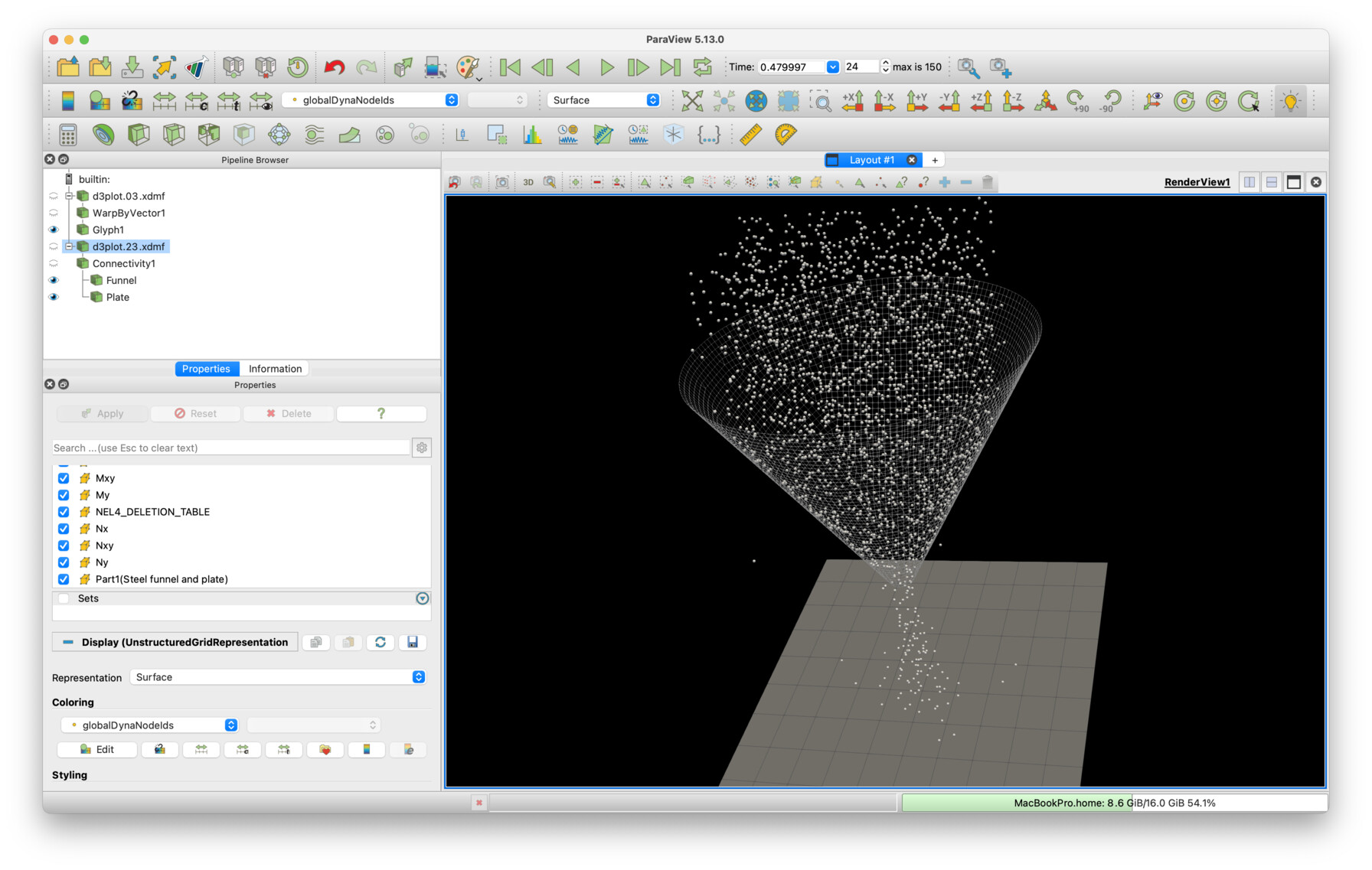
The state file can be downloaded here: funnelInjection.pvsm (1.1 MB)
Once the simulation with LS-DYNA is finished, we end up with these d3plot database files:
ll -h d3plot*
-rw-r--r--@ 1 larski  larski   2.6M Jul  8  2024 d3plot
-rw-r--r--@ 1 larski  larski   133M Jul  8  2024 d3plot01
-rw-r--r--@ 1 larski  larski   133M Jul  8  2024 d3plot02
-rw-r--r--@ 1 larski  larski   133M Jul  8  2024 d3plot03
-rw-r--r--@ 1 larski  larski   133M Jul  8  2024 d3plot04
-rw-r--r--@ 1 larski  larski   133M Jul  8  2024 d3plot05
-rw-r--r--@ 1 larski  larski   133M Jul  8  2024 d3plot06
-rw-r--r--@ 1 larski  larski   133M Jul  8  2024 d3plot07
-rw-r--r--@ 1 larski  larski   133M Jul  8  2024 d3plot08
-rw-r--r--@ 1 larski  larski   133M Jul  8  2024 d3plot09
-rw-r--r--@ 1 larski  larski   133M Jul  8  2024 d3plot10
-rw-r--r--@ 1 larski  larski   8.9M Jul  8  2024 d3plot11
-rw-r--r--@ 1 larski  larski   8.9M Jul  8  2024 d3plot12
The converter is simply invoked by
d3plot2hdf5 d3plot
which then produces this output
+--------------------------------------------------------------------+
|                                                                    |
| T A I L S I T                                                      |
| -------------                                                      |
|                                                                    |
| Program                 :: d3plot2hdf5                             |
| Purpose                 :: convert d3plot to h5/xdmf               |
| Build                   :: v0.10.0 [6fa1851]                       |
| Date                    :: Apr 28 2025,15:55:30                    |
| News, discussions, bugs :: https://discourse.tailsit.com           |
|                                                                    |
| Terms: https://tailsit.com/downloads/TAILSIT_B2B_GTC.pdf           |
|                                                                    |
| For non-commercial use only                                        |
|                                                                    |
| Copyright, 2025 by TAILSIT GMBH. All rights reserved.              |
| www.tailsit.com                                                    |
|                                                                    |
+--------------------------------------------------------------------+
Options:
  -- timeSteps:   all
  -- split files: false

Title/Part/Contact information:
  -- Header: Funnel Injection
  -- Parts:
     [mat-id:1] Steel funnel and plate
     [mat-id:2] DES
  -- Contacts: (NONE)

LS-DYNA files:
  -- "/home/larski/git/d3plot2hdf5/tests/dem/FunnelInjection/complete/d3plot"
  -- "/home/larski/git/d3plot2hdf5/tests/dem/FunnelInjection/complete/d3plot01"
  -- "/home/larski/git/d3plot2hdf5/tests/dem/FunnelInjection/complete/d3plot02"
  -- "/home/larski/git/d3plot2hdf5/tests/dem/FunnelInjection/complete/d3plot03"
  -- "/home/larski/git/d3plot2hdf5/tests/dem/FunnelInjection/complete/d3plot04"
  -- "/home/larski/git/d3plot2hdf5/tests/dem/FunnelInjection/complete/d3plot05"
  -- "/home/larski/git/d3plot2hdf5/tests/dem/FunnelInjection/complete/d3plot06"
  -- "/home/larski/git/d3plot2hdf5/tests/dem/FunnelInjection/complete/d3plot07"
  -- "/home/larski/git/d3plot2hdf5/tests/dem/FunnelInjection/complete/d3plot08"
  -- "/home/larski/git/d3plot2hdf5/tests/dem/FunnelInjection/complete/d3plot09"
  -- "/home/larski/git/d3plot2hdf5/tests/dem/FunnelInjection/complete/d3plot10"
  -- "/home/larski/git/d3plot2hdf5/tests/dem/FunnelInjection/complete/d3plot11"
  -- "/home/larski/git/d3plot2hdf5/tests/dem/FunnelInjection/complete/d3plot12"

LS-DYNA file information:
  -- Title:         Funnel Injection
  -- Version:       DEV
  -- Creation date: Mon Jul  1 09:18:32 2024
  -- Format:        double precision

Additional ASCII Data:
  -- NONE

State information:
  -- max. no. of states found:   152
  -- actual no. of states found: 152
  -- state range: [0:151]

Output written to:
  -- d3plot.03.xdmf
  -- d3plot.23.xdmf
  -- d3plot.h5

N O R M A L   T E R M I N A T I O N                  04/28/25 16:02:31
The converter took about 4 seconds to produce these files:
ll -h *.xdmf *.h5
-rw-rw-r-- 1 larski larski 1.4M Apr 26 07:38 d3plot.03.xdmf
-rw-rw-r-- 1 larski larski 1.3M Apr 26 07:38 d3plot.23.xdmf
-rw-rw-r-- 1 larski larski 1.5G Apr 26 07:38 d3plot.h5
All the heavy data is stored in the hdf5-file d3plot.h5 while the .xdmf files contain lightweight references to the .h5 file. The .xdmf files can then directly be processed by tools like ParaView.
The particle data is referenced from d3plot.03.xdmf while references to the structural data are stored in d3plot.23.xdmf.
Below is a tiny animation of the results. It displays the particles’ velocities through a period of roughly 2.8 seconds.

Scripting
A word on scripting. .xdmf stores references to the data in such a way that ParaView can digest the heavy data. However, it is the .h5 file that stores the data iteself. So, if you want to script your post-processing tasks it is a good idea to get accustomed to the structure of the .h5 file.
We recommend using command line tools to investigate the contents of the .h5 file. On Debian based systems those command line tools can be installed with
sudo apt install hdf5-helpers
Other Linux distributions supply the hdf5-helpers, too. Simply use the respective package manager. Alternatively, those tools are typically bundled with the binary distributions of HDF5. Simply go to
for further information. This destination might be helpful for Windows installations, too.
Once the hdf5 tools are installed you can work, e.g., with h5dump or h5ls. The latter gives you a condensed view of the contents while the output of h5dump can be rather exhaustive. In many ways the HDF5 format can be viewed as a kind of filesystem, and this is exactly how h5ls behaves like.
So, let’s get started. Calling
h5ls d3plot.h5 | column
is likely to produce this lengthy output:
annotation               Group	d3plot_stp025            Group	d3plot_stp051            Group	d3plot_stp077            Group	d3plot_stp103            Group	d3plot_stp129            Group
d3plot_stp000            Group	d3plot_stp026            Group	d3plot_stp052            Group	d3plot_stp078            Group	d3plot_stp104            Group	d3plot_stp130            Group
d3plot_stp001            Group	d3plot_stp027            Group	d3plot_stp053            Group	d3plot_stp079            Group	d3plot_stp105            Group	d3plot_stp131            Group
d3plot_stp002            Group	d3plot_stp028            Group	d3plot_stp054            Group	d3plot_stp080            Group	d3plot_stp106            Group	d3plot_stp132            Group
d3plot_stp003            Group	d3plot_stp029            Group	d3plot_stp055            Group	d3plot_stp081            Group	d3plot_stp107            Group	d3plot_stp133            Group
d3plot_stp004            Group	d3plot_stp030            Group	d3plot_stp056            Group	d3plot_stp082            Group	d3plot_stp108            Group	d3plot_stp134            Group
d3plot_stp005            Group	d3plot_stp031            Group	d3plot_stp057            Group	d3plot_stp083            Group	d3plot_stp109            Group	d3plot_stp135            Group
d3plot_stp006            Group	d3plot_stp032            Group	d3plot_stp058            Group	d3plot_stp084            Group	d3plot_stp110            Group	d3plot_stp136            Group
d3plot_stp007            Group	d3plot_stp033            Group	d3plot_stp059            Group	d3plot_stp085            Group	d3plot_stp111            Group	d3plot_stp137            Group
d3plot_stp008            Group	d3plot_stp034            Group	d3plot_stp060            Group	d3plot_stp086            Group	d3plot_stp112            Group	d3plot_stp138            Group
d3plot_stp009            Group	d3plot_stp035            Group	d3plot_stp061            Group	d3plot_stp087            Group	d3plot_stp113            Group	d3plot_stp139            Group
d3plot_stp010            Group	d3plot_stp036            Group	d3plot_stp062            Group	d3plot_stp088            Group	d3plot_stp114            Group	d3plot_stp140            Group
d3plot_stp011            Group	d3plot_stp037            Group	d3plot_stp063            Group	d3plot_stp089            Group	d3plot_stp115            Group	d3plot_stp141            Group
d3plot_stp012            Group	d3plot_stp038            Group	d3plot_stp064            Group	d3plot_stp090            Group	d3plot_stp116            Group	d3plot_stp142            Group
d3plot_stp013            Group	d3plot_stp039            Group	d3plot_stp065            Group	d3plot_stp091            Group	d3plot_stp117            Group	d3plot_stp143            Group
d3plot_stp014            Group	d3plot_stp040            Group	d3plot_stp066            Group	d3plot_stp092            Group	d3plot_stp118            Group	d3plot_stp144            Group
d3plot_stp015            Group	d3plot_stp041            Group	d3plot_stp067            Group	d3plot_stp093            Group	d3plot_stp119            Group	d3plot_stp145            Group
d3plot_stp016            Group	d3plot_stp042            Group	d3plot_stp068            Group	d3plot_stp094            Group	d3plot_stp120            Group	d3plot_stp146            Group
d3plot_stp017            Group	d3plot_stp043            Group	d3plot_stp069            Group	d3plot_stp095            Group	d3plot_stp121            Group	d3plot_stp147            Group
d3plot_stp018            Group	d3plot_stp044            Group	d3plot_stp070            Group	d3plot_stp096            Group	d3plot_stp122            Group	d3plot_stp148            Group
d3plot_stp019            Group	d3plot_stp045            Group	d3plot_stp071            Group	d3plot_stp097            Group	d3plot_stp123            Group	d3plot_stp149            Group
d3plot_stp020            Group	d3plot_stp046            Group	d3plot_stp072            Group	d3plot_stp098            Group	d3plot_stp124            Group	d3plot_stp150            Group
d3plot_stp021            Group	d3plot_stp047            Group	d3plot_stp073            Group	d3plot_stp099            Group	d3plot_stp125            Group	d3plot_stp151            Group
d3plot_stp022            Group	d3plot_stp048            Group	d3plot_stp074            Group	d3plot_stp100            Group	d3plot_stp126            Group	narbs                    Group
d3plot_stp023            Group	d3plot_stp049            Group	d3plot_stp075            Group	d3plot_stp101            Group	d3plot_stp127            Group
d3plot_stp024            Group	d3plot_stp050            Group	d3plot_stp076            Group	d3plot_stp102            Group	d3plot_stp128            Group
As you can see there are 152 time steps stored in d3plot.h5. If you now want to investigate a single time step a bit further you can do:
h5ls d3plot.h5/d3plot_stp000
which will give you:
fields03                 Group
fields23                 Group
grid03                   Group
grid23                   Group
gridXY stores the geometry information (or links to it), while fieldsXY stores the simulation data itself. Let’s investigate the latter a bit further. X denotes the reference dimension while Y denotes the dimension of the physical world. Hence, fields03 stores the particle data. Since this is the data we are interested in, we proceed with
h5ls d3plot.h5/d3plot_stp000/fields03
and obtain
cell                     Group
grid                     Group
node                     Group
These three groups denote to which entities the data is attached to. In a Finite Element simulation node would denote nodal or point data, cell would be element data, and grid would collect data such as energies or time series values which are global quantities that can neither be attached to a cell nor to a node.
Let’s assume we are further interested in the grid data. This time we invoke h5ls with the -r option which avoids further cycles and lists all groups recursively. So, entering
h5ls -r d3plot.h5/d3plot_stp000/fields03/grid
yields
/scalar                  Group
/scalar/internal\ energy(PART_0) Dataset {1}
/scalar/internal\ energy(PART_1) Dataset {1}
/scalar/internal\ energy(PART_ALL) Dataset {1}
/scalar/kinetic\ energy(PART_0) Dataset {1}
/scalar/kinetic\ energy(PART_1) Dataset {1}
/scalar/kinetic\ energy(PART_ALL) Dataset {1}
/scalar/mass(PART_0)     Dataset {1}
/scalar/mass(PART_1)     Dataset {1}
/scalar/time             Dataset {1}
/scalar/total\ energy(PART_0) Dataset {1}
/scalar/total\ energy(PART_1) Dataset {1}
/scalar/total\ energy(PART_ALL) Dataset {1}
/vector                  Group
/vector/rigid\ body\ velocity(PART_0) Dataset {3}
/vector/rigid\ body\ velocity(PART_1) Dataset {3}
/vector/rigid\ body\ velocity(PART_ALL) Dataset {3}
This time we get to the data itself. We can see that grid contains a scalar and a vector group. So, if we are interested in the energies over time we now know exactly where the data of interest is stored. Clearly, you do not need to process the data soley with h5ls. You could also use software packages like, e.g., octave, Matlab, or Mathematica to accomplish this task. Feel free in the choice of your tools. And if you want to use a freely available tool that provides a graphical user interface we recommend HDFView.
Finally, this scripting section would be rather incomplete without a script itself. Now that we know the structure of the .h5 file we can create a simple Python-script that plots the energies over time. The script looks like:
#!/usr/bin/env python3

import h5py
import re
import matplotlib.pyplot as plt
import numpy as np
import sys

def extract_data( h5file: str, part: str ):
    data = []
    with h5py.File( h5file, 'r' ) as f:
        group_names = list(f.keys())

        pattern = re.compile( r'^d3plot_stp\d{3}$')
        for group_name in group_names:
            if pattern.match(group_name):
                base = f"/{group_name}/fields03/grid/scalar"
                # time
                time = f"{base}/time"
                # kinetic energy
                ke = f"{base}/kinetic energy({part})"
                # internal energy
                ie = f"{base}/internal energy({part})"
                # total energy
                te = f"{base}/total energy({part})"
                t = f[time][:][0]
                kw = f[ke][:][0]
                iw = f[ie][:][0]
                tw = f[te][:][0]
                data.append( [t, kw, iw, tw] )
    return np.array(data)

def plot( data, part ):
    t  = data[:,0]
    kw = data[:,1]
    iw = data[:,2]
    tw = data[:,3]

    plt.figure(figsize=(12,8))

    plt.plot(t,tw,marker='o', linestyle='-',color='b',label='Total')
    plt.plot(t,iw, linestyle='-',color='g',label='Internal')
    plt.plot(t,kw, linestyle='-',color='m',label='Kinetic')
    plt.xlabel('time [s]')
    plt.ylabel('energy')
    plt.title(f'Energies over time [{part}]')
    plt.grid(True)
    plt.legend()
    plt.savefig(f'energy_{part}.png', format='png', dpi=300)
    plt.show()


if __name__ == "__main__":
    try:
        if len(sys.argv) is not 3:
            raise ValueError(f"Usage: {sys.argv[0]} h5-file part, part = 0|1|ALL")
        #
        # PARSE COMMAND LINE
        h5file = sys.argv[1]
        part = "PART_"
        part = f"{part}{sys.argv[2]}"
        #
        ## EXTRACT DATA
        data = extract_data( h5file, part )
        #
        # PLOT DATA
        plot(data,part)
        #
        # DONE
    except ValueError as e:
        print( f"An error has ocurred: {e}")
The script can be downloaded here:
processEnergies.py (2.0 KB)
And the required packages can be found herein:
requirements.txt (255 Bytes)
Calling
python3 -m venv venv
source venv/bin/activate
pip3 install -r requirements.txt
./processEnergies.py d3plot.h5 ALL
then produces the following plot
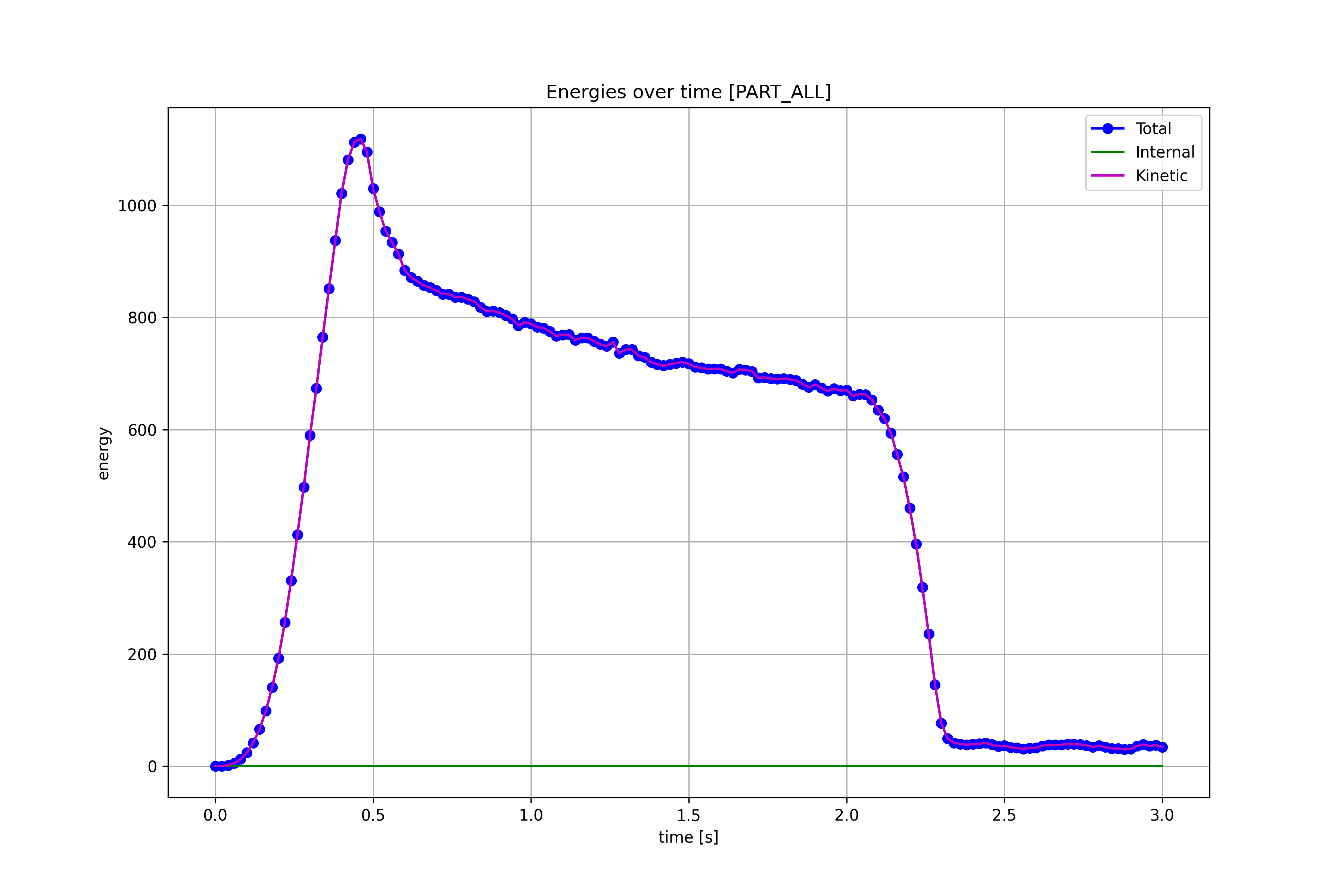
That’s it!